- Published on
A Hierarchical Bayesian Model for Separating Trader Skill from Luck
Crypto "top trader" leaderboards rank wallets by raw return. But return over a handful of trades is almost all noise: a wallet that is +300% after five trades is, overwhelmingly, lucky. Copy it and you are copying a coin flip.
The real task is to estimate a trader's latent skill — the part that persists — from a noisy, finite sample of trades, and to quantify how sure we are. The difference between "+3% ± 0.2%" and "+3% ± 4%" is the difference between a signal and a mirage. That is exactly what a hierarchical Bayesian model is for.
This post walks through the whole thing: how the data is collected and filtered, why partial pooling is the right idea, the closed-form conjugate updates that let the model learn online, the full hierarchical fit in PyMC, and a single continuous walk-forward that tests whether the learned skill actually predicts who is worth copying. It does — and then an honest autopsy shows exactly where that edge came from.
TL;DR
- Data: ~93 hours of the Hyperliquid perpetuals tape — 7.6M trades, 178 coins, ~64k wallets — reconstructed into per-trader position returns.
- Model: a hierarchical Bayesian model gives each trader a posterior mean edge and Sharpe ratio with a credible interval, shrinking thin-data traders toward "no edge" so a lucky five-trade wallet is not mistaken for a skilled one.
- It predicts out-of-sample (walk-forward, no lookahead): the live skill estimate forecasts a trader's next position (Spearman ρ = +0.21), and traders it flags as skilled earn +0.44%/position gross going forward.
- It beats the alternatives: of the traders it calls skilled, 70% are profitable next (vs. 43% for a profit-threshold rule, 32% for random). In an online, walk-forward top-10 copy account, ranking traders by learned skill yields 77% winning copies (+9.3%) vs. 54% (+8.5%) for ranking by realized profit — at a third of the drawdown, both far above random (−1.0%).
- But the edge is concentrated: an autopsy shows ~76% of that return came from a single trending asset. The method is sound; the market window was kind.
The bulk of this post is about the data, the filtering, and the model — that is the interesting part.
1. The problem: skill vs. luck
Skill is the component of a trader's results that persists into the future; luck is the component that does not. With only a handful of trades, the two are hopelessly entangled in the raw average — a few outsized wins can carry a mediocre trader to the top of a leaderboard, and a few unlucky losses can bury a good one.
So the question is not "what was this wallet's return?" but "what is the best estimate of the return it will keep delivering, and how confident can we be?" Answering that well requires three things at once: a way to borrow strength across the whole population of traders (so we are not fooled by tiny samples), a way to separate signal from noise explicitly, and a way to report uncertainty rather than a single point estimate. A hierarchical Bayesian model delivers all three.
2. The data — how it is collected and filtered
Source & collection. A lightweight collector subscribes to the Hyperliquid websocket and records every fill on every perpetual market — timestamp, coin, price, size, side, and the buyer and seller wallet addresses. This study uses one continuous ~93-hour stream: 7,610,323 trades, 178 coins, ~63,700 distinct wallets (45,957 of them with at least one completed position).
From fills to position returns. Skill is naturally per position, not per fill. For each wallet we replay their fills with average-cost accounting and emit one record per closed position (an independent entry → exit round trip), taking its return on deployed capital r = PnL / entry_notional, winsorized to ±25% to tame fat tails. These per-position returns are the observations the model sees. (Each position is a round trip, so we use "trade" and "position" interchangeably below.)
Filtering to "serious retail." Not every wallet is a copy candidate. We keep wallets whose median position notional is $1,000–$5,000:
- below this band sit dust accounts whose results are pure noise;
- above it sit market-makers and funds whose edge is the bid/ask spread — which a copier crossing the spread cannot capture.
A size-band sweep confirmed this $1k–$5k band carries the most copyable skill. We then apply a minimum-activity filter on top (a trader needs some history to be judged): ≥5 positions → 1,387 traders (the population fit), ≥6 → 1,121 (the backtests), ≥8 → ~1,000 (the full hierarchical fit), ≥10 → 528 (the metric test).
Costs. A round-trip taker fee of 0.09% is charged once per position everywhere below — the hurdle skill must clear.
3. The model
The model is a three-level hierarchy — population → trader → trade. Reading downward is the generative story (how the data is born); reading upward is inference (learning each trader's skill from their trades). Skill is the per-trader Sharpe ratio μᵢ / σᵢ.
We build it in two layers; the second generalizes the first.
3.1 Partial pooling — the core idea
Every trader's data is a small, noisy sample. Two naive options are both wrong: no pooling (trust each raw average — overfits lucky small samples) and complete pooling (assume everyone is the population average — ignores real skill). A hierarchical model does partial pooling: it puts all traders under a shared prior and makes each estimate a precision-weighted compromise between the trader's own data and the crowd — pulled hard toward the crowd when data is thin, barely when it is rich.
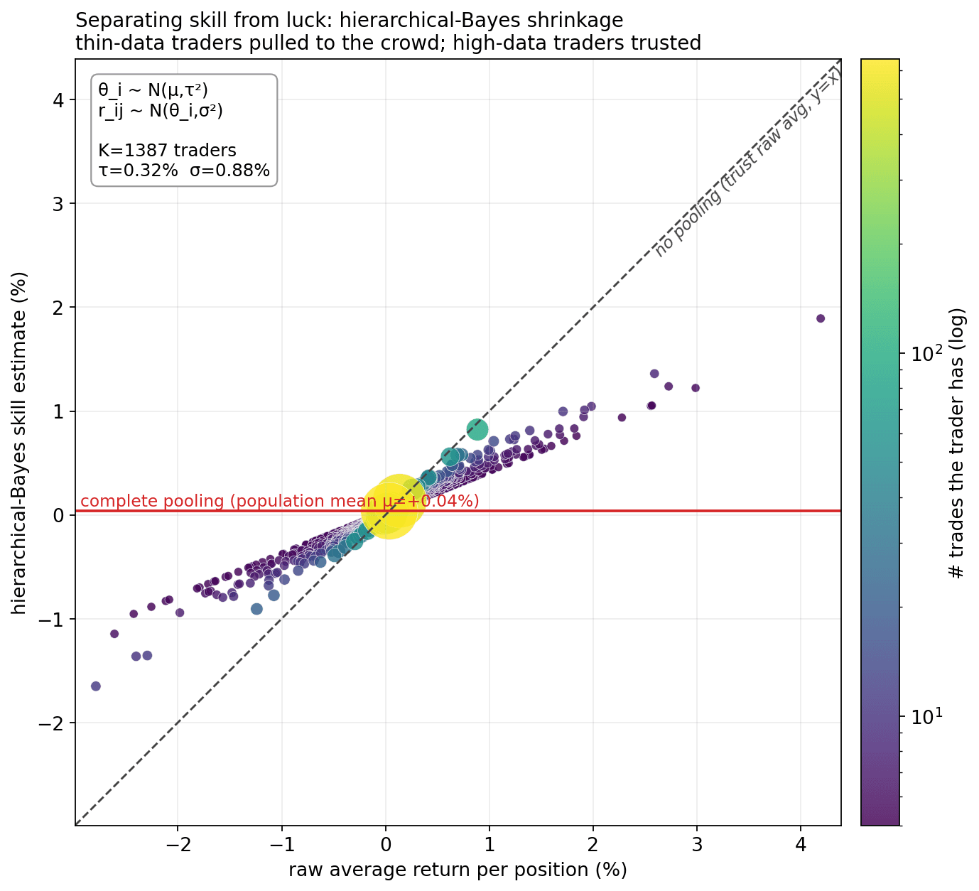
Each dot is one of 1,387 traders (≥5 positions): raw average return (x) vs. the model's skill estimate (y), coloured and sized by number of positions. Thin-data traders are yanked toward the population mean (their gaudy averages are mostly luck); high-data traders sit near the diagonal. This is the signature picture of a hierarchical model.
3.2 Model v1 — per-trader mean (Normal–Normal)
The first model treats skill as the mean per-trade return θᵢ:
θ_i      ~ Normal(μ, τ²)          # population of trader skills    (the prior)
r_ij|θ_i ~ Normal(θ_i, σ²)        # a trader's trades = skill + noise   (the likelihood)
μ is the crowd's edge, τ the between-trader skill spread (signal), σ the within-trader per-trade noise (luck). Because Normal–Normal is conjugate, the per-trader posterior is closed-form — no sampling. After k trades with sample mean r̄:
posterior precision  = 1/τ² + k/σ²
θ̂_i (posterior mean) = (μ/τ² + k·r̄/σ²) / (1/τ² + k/σ²)
posterior sd         = sqrt(1 / (1/τ² + k/σ²))
The posterior mean is a precision-weighted blend of crowd μ and data r̄; the data weight k/σ² ÷ (1/τ² + k/σ²) is the reliability of a k-trade record (it grows from ~0 to ~1).
How v1 is "trained." There is no gradient descent — for a conjugate model, training is exact Bayesian updating. We need only μ, τ, σ, estimated by empirical Bayes (the crowd sets its own prior; τ² via the DerSimonian–Laird moment estimator). On this data: μ ≈ +0.04%/position, τ ≈ 0.32%, σ ≈ 0.88% — a signal-to-noise ratio of τ/σ ≈ 0.37. Skill is real but small relative to per-trade noise, which is exactly why naive averages over a few trades mislead. For decisions we use a fixed skeptical prior (μ = 0, small τ₀) and flag on P(θᵢ > fee) = Φ((θ̂ᵢ − fee)/sd).
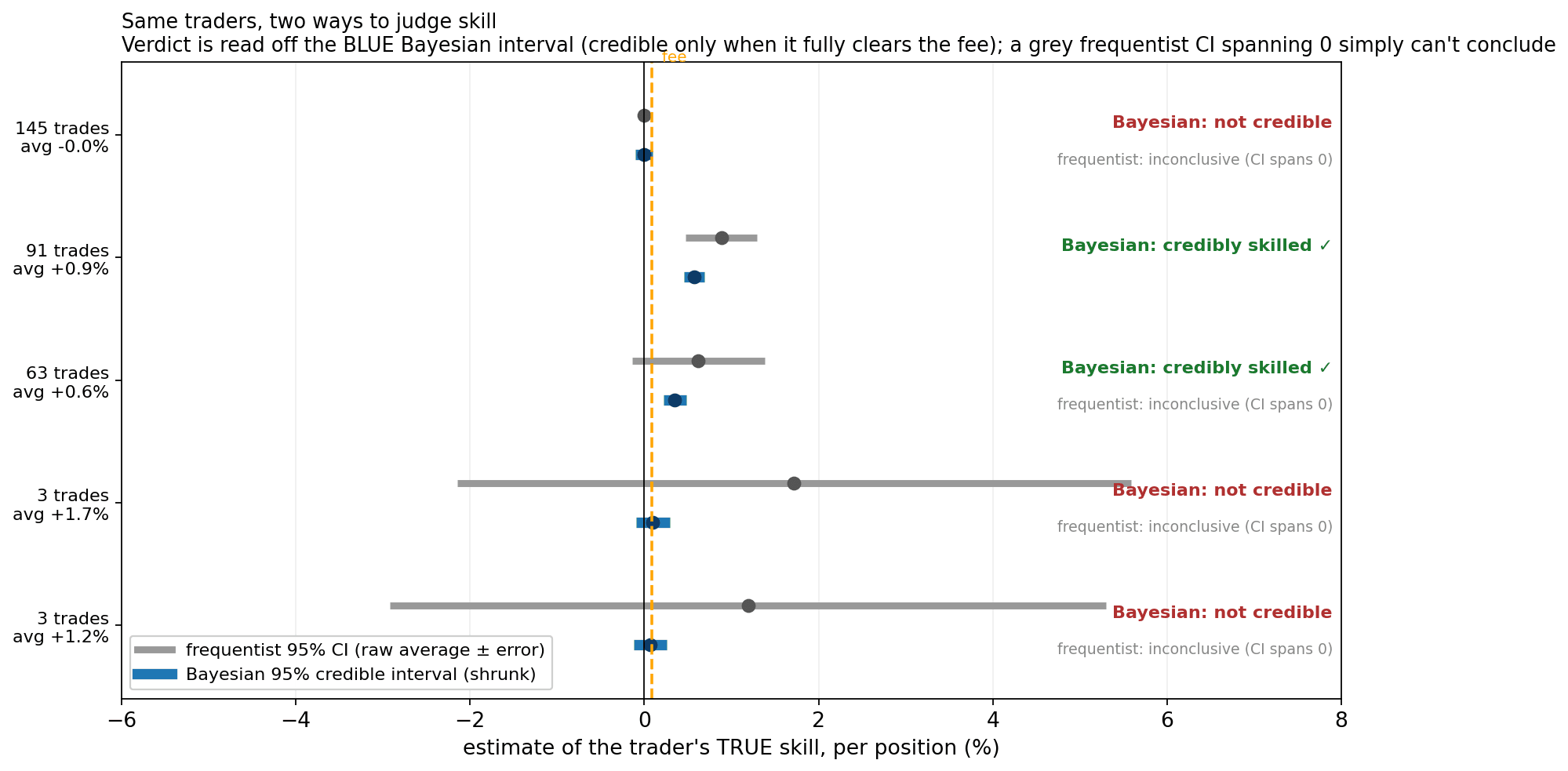
Decision-ready: a few real traders shown as a frequentist 95% CI (raw average, grey) vs. a Bayesian 95% credible interval (shrunk, blue). The verdict is read off the blue Bayesian interval — a trader is called credibly skilled only when that interval lies entirely above the fee (hence above zero). The grey frequentist CI is shown alongside: on a 3-trade wallet it is so wide it is useless, and even on the 63-trade trader it spans zero — so the frequentist test cannot conclude skill, while the shrunk Bayesian interval can. Note the discipline: the 5-trade, +2.3% wallet has a Bayesian interval barely above zero but below the fee, so it is correctly not flagged — a bare "above zero" rule would wrongly chase that luck.
3.3 Model v2 — per-trader mean and variance; skill = Sharpe
Mean alone ignores risk: two traders with the same average but different volatility are not equally skilled — the steadier one sizes larger (Kelly ∝ μ/σ²) and survives. Model v1's weakness is a single shared σ. So v2 gives each trader their own variance and defines skill as the Sharpe ratio Sᵢ = μᵢ / σᵢ. For one trader, the conjugate model for unknown mean and variance is the Normal–Inverse-Gamma, with a closed-form streaming update after n trades (mean x̄, M₂ = Σ(x−x̄)²):
κₙ = κ₀ + n      μₙ = (κ₀·μ₀ + n·x̄)/κₙ
αₙ = α₀ + n/2    βₙ = β₀ + ½·M₂ + ½·κ₀·n·(x̄−μ₀)²/κₙ
The marginal of μ is Student-t; σ² ~ InvGamma(αₙ, βₙ). The posterior Sharpe comes from sampling σ² ~ InvGamma, μ ~ Normal | σ², and computing μ/σ. Streamed over one real trader, walk-forward — flag the instant the Sharpe is credibly positive, then keep following:
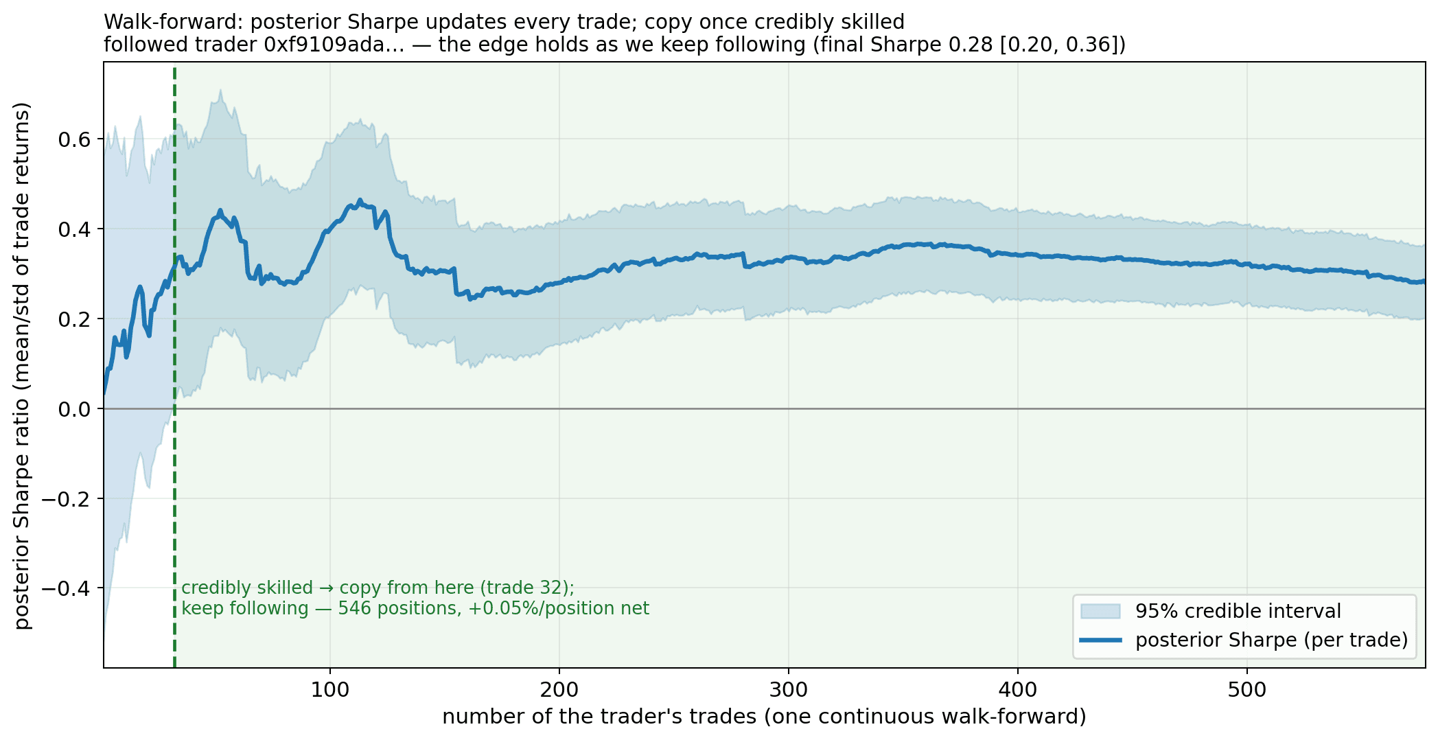
One trader. The 95% posterior Sharpe interval straddles zero for ~30 trades (we do not trust them), clears zero around trade 32 → we start copying, and the posterior Sharpe holds steady the rest of the stream. It is one continuous walk-forward — there is no period boundary. The point is the method (flag, then follow), not this one trader's (thin) edge.
3.4 Training the full hierarchical model — step by step
To pool the per-trader variances too, we put a hierarchical prior on both the mean and the log-volatility. That breaks conjugacy (a log-normal prior on σ has no closed form), so here we use probabilistic programming: write the generative model in PyMC and sample the posterior.
Step 0 — Generative story. A Bayesian model is a recipe for simulating data: (1) the world has μ_pop, τ_μ, m_logσ, s_logσ; (2) each trader draws μᵢ ~ N(μ_pop, τ_μ) and σᵢ = exp(N(m_logσ, s_logσ)); (3) each trade is rᵢⱼ ~ N(μᵢ, σᵢ); (4) skill is Sᵢ = μᵢ/σᵢ. Inference runs it backwards. We model log σ because volatility is positive and multiplicative.
Step 1 — Priors (weakly informative, skeptical): μ_pop ~ N(0, 0.003) (edge centered at zero), τ_μ ~ HalfNormal(0.003), m_logσ ~ N(log 0.007, 0.5), s_logσ ~ HalfNormal(0.5). Scales are HalfNormal (positive-only). Tight enough to regularize ~1,000 noisy traders; loose enough to let the data move them.
Step 2 — Prior predictive check. Sample returns from the priors and confirm they are plausible (a few tenths of a percent to a couple of percent per trade) before fitting.
Step 3 — Reparameterize (the funnel). Writing μᵢ ~ N(μ_pop, τ_μ) directly creates Neal's funnel — when τ_μ is small the geometry pinches and a single-step-size sampler stalls. The fix is the non-centered form: sample a unit-normal offset and scale it (μᵢ = μ_pop + z·τ_μ), for both μᵢ and log σᵢ. Without it a hierarchy like this will not mix.
Step 4 — The model:
import pymc as pm
from numpy import log

with pm.Model(coords={"trader": traders}) as model:
    mu_pop = pm.Normal("mu_pop", 0.0, 0.003)                  # population edge (skeptical)
    tau_mu = pm.HalfNormal("tau_mu", 0.003)                   # between-trader spread
    m_ls   = pm.Normal("m_logsig", log(0.007), 0.5)          # population log-volatility
    s_ls   = pm.HalfNormal("s_logsig", 0.5)
    zmu = pm.Normal("zmu", 0, 1, dims="trader")              # non-centered offsets
    zls = pm.Normal("zls", 0, 1, dims="trader")
    mu     = pm.Deterministic("mu",     mu_pop + zmu*tau_mu,          dims="trader")
    sigma  = pm.Deterministic("sigma",  pm.math.exp(m_ls + zls*s_ls), dims="trader")
    sharpe = pm.Deterministic("sharpe", mu/sigma,                     dims="trader")  # the skill
    pm.Normal("obs", mu=mu[idx], sigma=sigma[idx], observed=y)   # idx maps each trade -> its trader
    idata = pm.sample(1000, tune=1500, chains=4, target_accept=0.95)
coords/dims keep posterior arrays labelled per-trader; pm.Deterministic("sharpe", …) records the full posterior over the Sharpe for free; mu[idx] is the vectorized likelihood; PyMC builds a computation graph with exact gradients by autodiff.
Step 5 — Run NUTS. Sampling uses NUTS (No-U-Turn Sampler), adaptive Hamiltonian Monte Carlo: give the point momentum and simulate physics (a leapfrog integrator on the gradients) to a distant, low-correlation proposal; the no-U-turn rule auto-stops each trajectory. During warmup (tune, discarded) the step size is adapted to target_accept=0.95 (high, to suppress divergences) and a mass matrix is estimated. We ran 4 chains × (1500 + 1000) = 4,000 draws.
Step 6 — Convergence diagnostics (honest). R̂ (chain agreement, want <1.01) came in ~1.01–1.03; ESS (independent-draw count) is low on a few per-trader parameters. Verdict: solid at the population level, marginal for individual low-data σᵢ — expected, since a trader with 8 trades barely identifies their own variance. (For production: more draws, target_accept=0.99, a Student-t likelihood for the tails.)
Step 7 — Posterior predictive check. Simulate from the fitted posterior and compare to the real trades; the Normal likelihood mildly under-covers the extreme tails (hence Student-t on the to-do list).
Step 8 — Read off the answer. sharpe is a tracked deterministic quantity, so the fit contains a full posterior of every trader's Sharpe; summarize each with a posterior mean and 95% credible interval.
Why we can also stream it. The walk-forward needs the posterior at every trade with no lookahead. The Normal–Normal / Normal–Inverse-Gamma updates are exact in closed form by conjugacy (a theorem), so we sample the rich hierarchy for the forest below and stream the closed-form update for every walk-forward decision.
3.5 What it gives us: a posterior Sharpe per trader
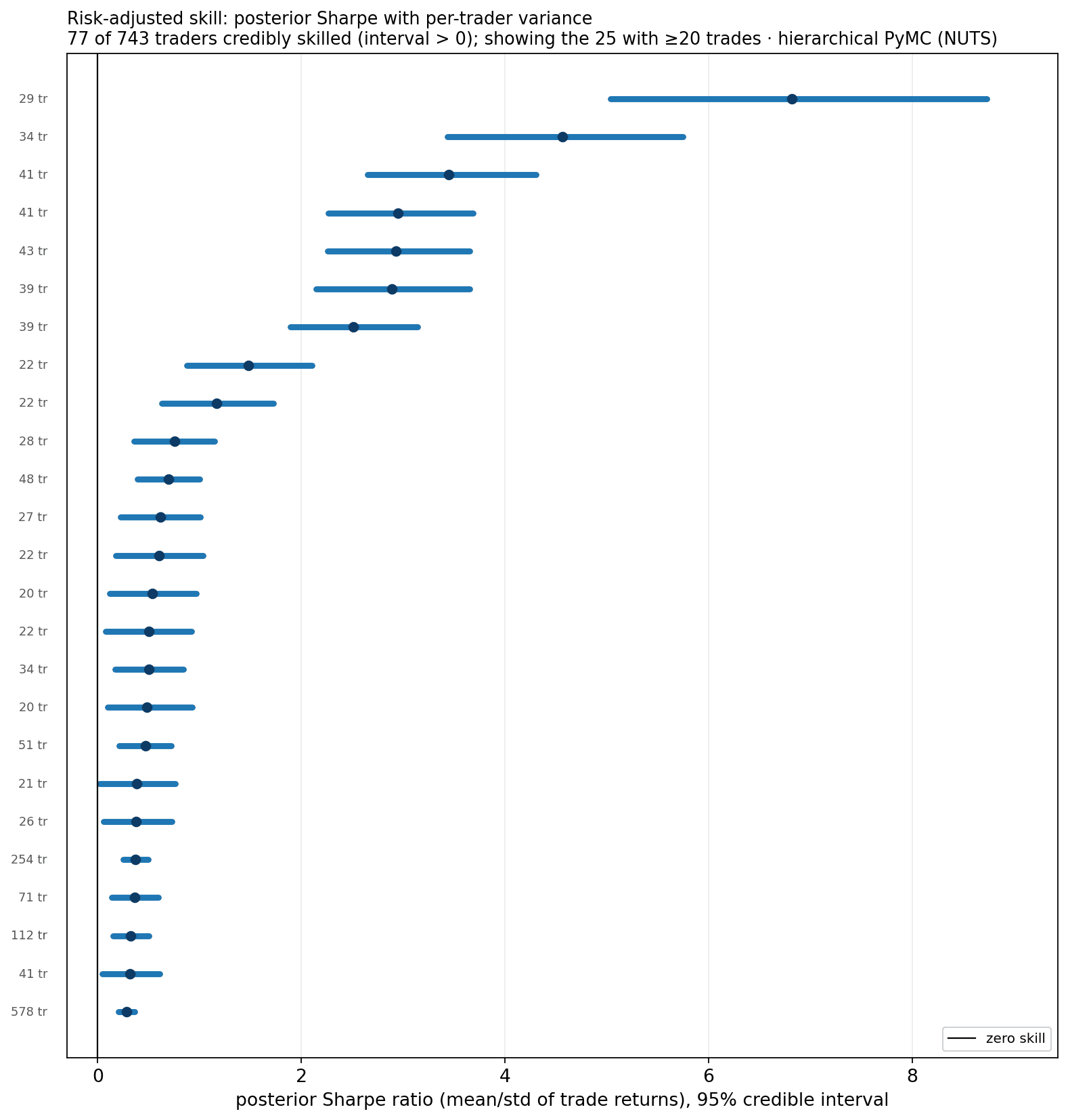
Posterior Sharpe ratio with 95% credible intervals — 77 of 743 traders are credibly skilled (interval clears zero), showing the credibly-skilled traders with ≥20 trades for legibility. What feeds it: a single batch fit over every position in the window — all 17,724 positions of the 743 traders (≥8 positions each; median 12, max 645 per trader), so each trader's interval uses their complete record. Because a Bayesian posterior conditioned on all of a trader's trades is the same whether updated one-at-a-time or in one batch, this is exactly the all-trades ("final") posterior — the full-information skill verdict, in contrast to the no-lookahead walk-forward of §5, which reads the same posterior at each earlier decision point. Note the pattern: traders with hundreds of trades have tight intervals at a modest Sharpe (certain, modest edge), while 40-ish-trade traders show a higher Sharpe with wider intervals.
4. Which definition of skill? An empirical test
We did not assume Sharpe is best — we split each trader's trades in half and asked which definition of skill, measured on the first half, best predicts the held-out half.
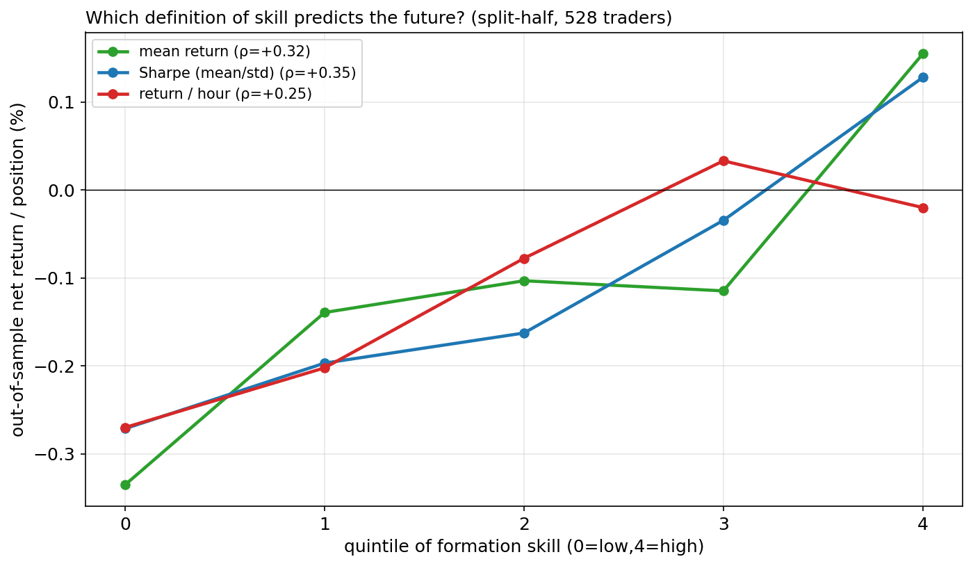
All three predict the held-out half (rank correlation ρ ≈ 0.25–0.35). Mean maximizes raw forward return; Sharpe (mean/std) is the best ranker (ρ = +0.35) and the steadiest; return-per-hour loses because per-position fees punish the fast scalpers it favours. We keep Sharpe — robust, and it feeds position sizing directly (Kelly ∝ μ/σ²).
5. Does it work? One continuous walk-forward
Everything here is walk-forward: the posterior is computed only from trades before each decision, and we measure what happens after. No lookahead.
5.1 The estimate predicts the next trade
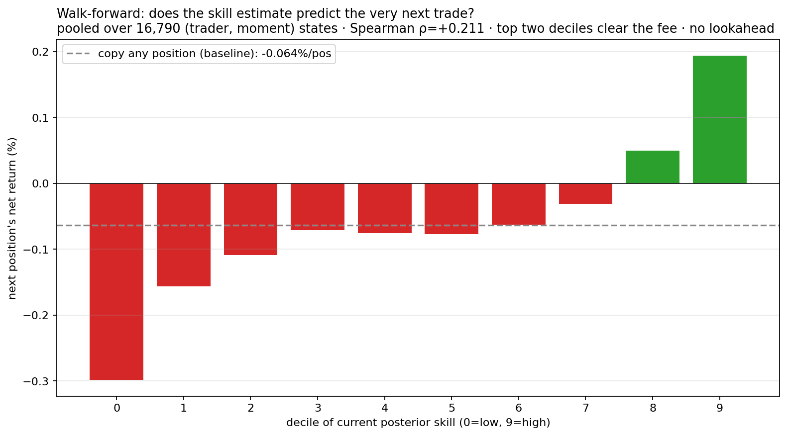
At every point in every trader's stream, pair the current posterior skill with the next position's return. Pooled over 16,790 (trader, moment) states, higher skill → higher next-trade return — Spearman ρ = +0.21. Only the top two deciles clear the fee; the rest lose.
5.2 It beats a profit threshold, a frequentist test, and random
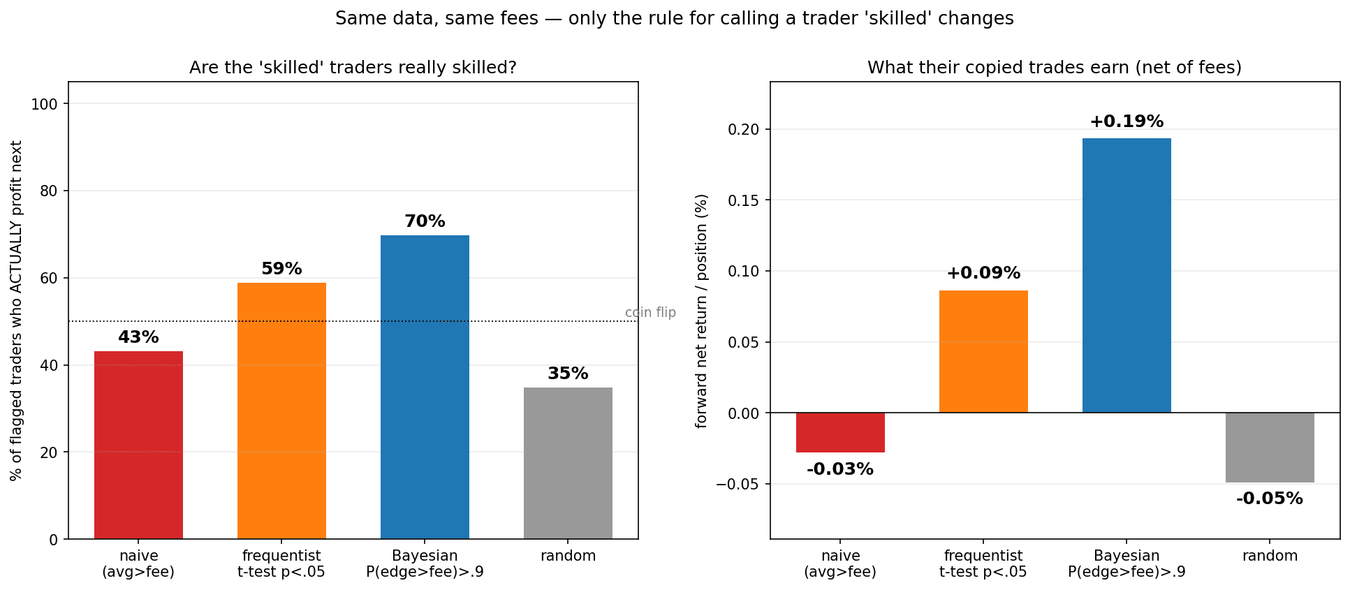
Same data, same fees — only the rule for calling a trader "skilled" changes:
| Rule | flagged traders who profit next | forward net return/position |
|---|---|---|
| Random | 32% | −0.12% |
| Profit threshold ("avg > fee") | 43% | −0.03% |
| Frequentist t-test (p<.05) | 59% | +0.09% |
| Bayesian (P(edge>fee)>0.9) | 70% | +0.19% |
The Bayesian rule wins because it shrinks small samples and only commits at high posterior probability — and it returns a posterior probability of skill, which a t-test's accept/reject is not.
5.3 Flagged traders keep winning (event study vs. random)
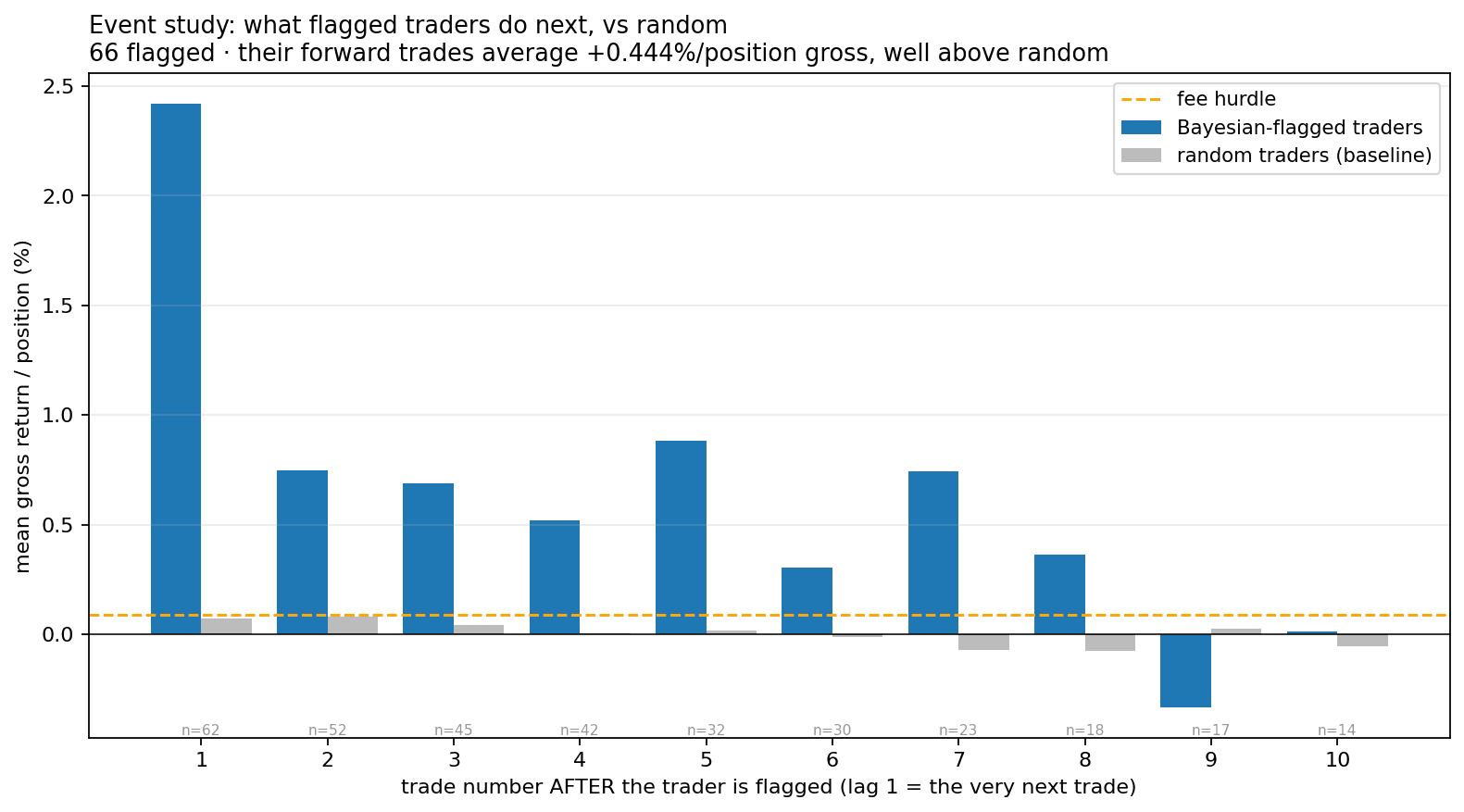
When the model flags a trader, their subsequent positions average +0.44% gross — far above random traders (grey) and the fee, from the very next position onward. We copy every position they open after the flag.
5.4 Copying the top traders: rank by realized profit, or by learned skill?
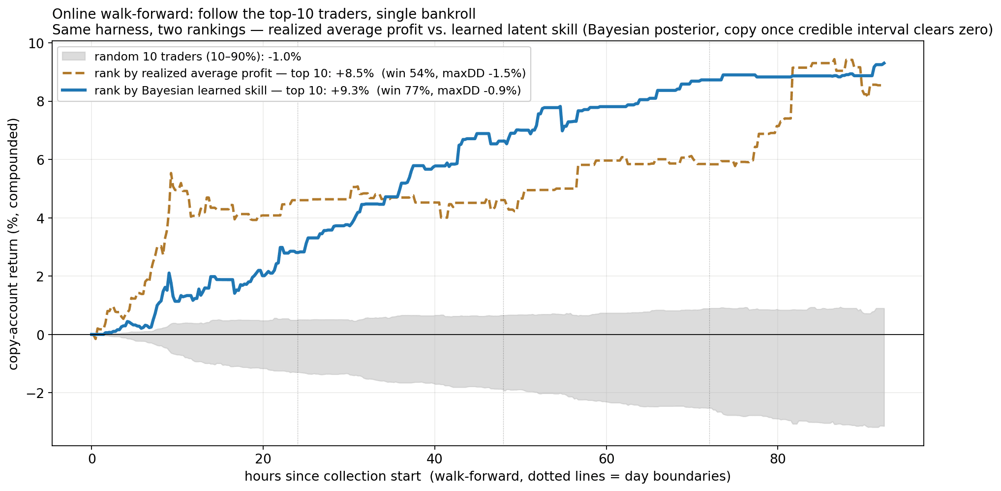
The realistic test. We run the whole thing online, walk-forward: every trader is updated trade-by-trade from collection start, and at any moment we copy only the top 10 traders — under two competing rankings. One ranks traders by their realized average profit so far; the other ranks by Bayesian learned skill (the posterior) and only starts copying a trader once its credible interval clears zero. Identical universe, identical single bankroll (10% of equity per copied position, net of fee), identical cap of ten — only the ranking differs.
Ranking by learned skill returns +9.3% vs. +8.5% for ranking by realized profit (a random ten: −1.0%). The extra return is modest; the real difference is quality. 77% of the learned-skill copies are winners, vs. 54% for realized profit — at a third of the drawdown (−0.9% vs. −1.5%). Ranking by realized profit chases hot hands: it sprints out early (it copies a trader the instant they look profitable, lucky ones included) and pays for it in choppiness. Ranking by learned skill waits for the evidence, then copies traders who keep winning — three of every four copied positions pay.
5.5 Why learn skill instead of just averaging? A small-sample phenomenon
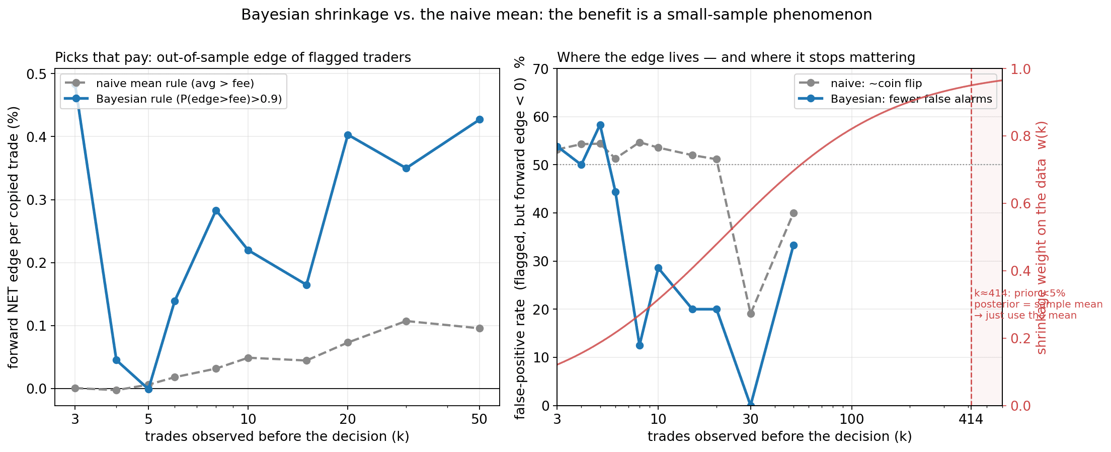
The Bayesian machinery earns its keep precisely when data is thin. Give two rules the same first k trades and score their picks out-of-sample (left): the plain "average beats the fee" rule flags about half the field with a ~50% false-positive rate — a coin flip — and ~0% forward edge, because at small k an average is mostly luck. The learned-skill rule, which shrinks lucky streaks toward zero, flags far fewer but with positive forward edge and a far lower false-positive rate.
And it says exactly when it stops mattering (right). The posterior is a precision-weighted blend of the skeptical prior and the data, with a data weight w(k) that climbs from 0 toward 1 — crossing 0.5 at k≈22 trades and 0.95 at k≈414. Past a few hundred trades the prior contributes <5%, the posterior equals the sample mean, and the two rules converge. So the Bayesian edge is a genuine small-sample phenomenon: it matters most for the thin-record traders who make up almost the entire field (the median trader here has 9 positions), and it gracefully reduces to "just use the average" once a trader has hundreds of trades.
5.6 Where did the return come from? A per-coin autopsy
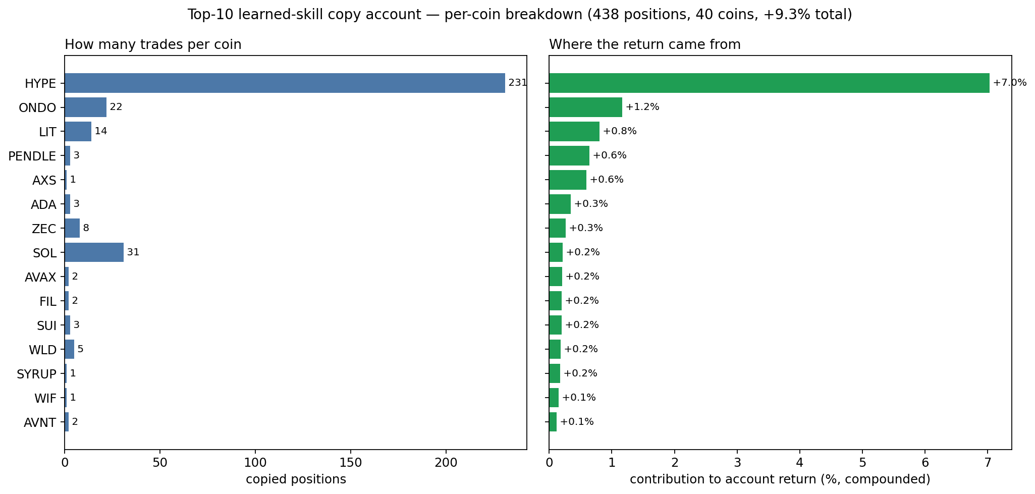
Aggregate numbers hide concentration, so we attributed every one of the 438 copied positions back to its coin. The result is sobering: the account is essentially one trade. HYPE alone is 231 positions (53% of all copies), a 96% win rate, and +7.0% — 76% of the entire +9.3% return; the top five coins account for ~110% of the gains (the rest roughly net to zero). Tellingly, the same "skilled" traders lose money on the majors — BTC (27 positions, 30% win, −0.5%) and ETH (16 positions, 44% win, −0.5%). During this window Hyperliquid's own token HYPE had a strong directional run, and the traders the model flags were largely riding it. A 96% win rate is not coin-agnostic trading skill — it is concentration in one trending asset, and it is exactly the kind of thing the headline +9.3% / 77%-win figure conceals.
6. Honest caveats
- ~93 hours of one continuous stream. The walk-forward evidence is strong and out-of-sample, but it is still one market window; a longer stream would tighten every estimate.
- Thin per-trade edge, but a high hit-rate. A flagged trader's forward edge is ~+0.44%/position gross → ~+0.19% net of the fee — small per position, but reliable: an online top-10 copy account ranked by learned skill wins on 77% of copied positions and compounds to ~+9% over ~4 days at 10%/position sizing (the level scales with the sizing/leverage knob; gains are somewhat concentrated in a minority of traders).
- MCMC convergence is marginal on individual low-data σᵢ (R̂ up to ~1.03). Population conclusions are sound; a production fit would use more draws, higher
target_accept, and a Student-t likelihood. - The edge is concentrated, not diversified (§5.6). ~76% of the copy account's return — and a 96% win rate — comes from HYPE during a strong directional run; the same flagged traders lose on BTC and ETH. So the result is partly "the model finds traders who were long the right trending asset," which is regime- and asset-specific and may not generalize to a flatter market.
- Modelling simplifications. Winsorization at ±25%, a Normal (not heavy-tailed) likelihood, market-makers excluded, and reconstructed PnL slightly inflates wallets holding a position before collection began.
7. Conclusion
A trader's raw return is mostly luck. A hierarchical Bayesian model — partial pooling, per-trader mean and variance, skill as a posterior Sharpe ratio — separates the skill from the luck, reports honest uncertainty, learns online in closed form, and (where conjugacy breaks) trains by NUTS in minutes. In one continuous walk-forward it predicts the next trade (ρ = +0.21), beats a profit-threshold rule, a frequentist test, and random selection (70% vs. 32% of picks profitable), and — ranking traders by learned skill rather than realized profit — drives an online top-10 copy account to +9.3% with 77% winning copies (vs. +8.5% / 54% for profit-ranking, and −1.0% for random).
The autopsy keeps us honest: most of that return rode one trending asset, so the headline figure says as much about the window as the method. But the core claim survives it. Skill is real, it is learnable from a modest number of trades, and the discipline that makes it learnable — shrink the lucky streaks, quantify the uncertainty, and commit only when the evidence clears the fee — is exactly what a hierarchical Bayesian model is built to do.